Here's a 4-week, visual-first learning plan to master Transformer architecture, LLMs, and GPTs, tailored for visual learners.

Interactive Websites

• Colab Study Notes - Sree+Vizuara
• Learn DNN Sree Hugging Face
• https://huggingface.co/spaces/schogini/llm-token-explorer
• https://poloclub.github.io/transformer-explainer/
• https://huggingface.co/spaces/schogini/GPT-2-Token-Inspector-Self-Attention
• https://nlp.seas.harvard.edu/annotated-transformer/
• https://huggingface.co/spaces/schogini/transformer-introduction
• https://huggingface.co/spaces/rahideer/Transformer

Videos and Channels

Activation Functions - EXPLAINED!

Self-Attention Using Scaled Dot-Product Approach

Multi-Head Attention Visually Explained

Self-Attention Using Scaled Dot-Product Approach

Feed forward neural networks

Attention in transformers, step-by-step | DL6

Transformers in Deep Learning | Introduction to Transformers

Coding Transformer From Scratch With Pytorch in Hindi Urdu || Training | Inference || Explanation

Multi-headed attention

The math behind Attention: Keys, Queries, and Values matrices

EASIEST Way to Train LLM Train w/ unsloth (2x faster with 70% less GPU memory required)

Attention in transformers, step-by-step | DL6

From Attention to Generative Language Models - One line of code at a time!

Finetune LLMs to teach them ANYTHING with Huggingface and Pytorch | Step-by-step tutorial

	Building LLMs from the Ground Up: A 3-hour Coding Workshop
	Lecture 1: Building LLMs from scratch: Series introduction

https://sebastianraschka.com/pdf/slides/2024-build-llms.pdf

Week 1: Foundations of Neural Networks & Attention

Goal: Build core understanding of neural nets, embeddings, and attention.

Week 2: The Transformer Architecture Deep Dive

Goal: Understand each block—embedding, attention, feed-forward, positional encoding.

Week 3: GPT, BERT, and Friends

Goal: Understand GPT-like models, masked language modeling, causal attention.

Week 4: Interact, Visualize, and Build

Goal: Simulate and build something visual from what you’ve learned.

Would you like me to package this plan as a downloadable PDF or Notion template with all links embedded?

For a visual learner, the best way to learn Transformer architecture, LLMs, and GPTs is through structured, visual-first resources that blend intuition with animations, diagrams, and interactive tools. Here's a curated path:

1. Foundation via Visual Intuition

• Animated Videos:

  • 3Blue1Brown’s Neural Network series (for neural net basics).

  • Jay Alammar's YouTube and blog:

  • Blog: The Illustrated Transformer

  • Video: Visual Introduction to Transformers

• Papers with Code – Visualizations:

  • https://paperswithcode.com/method/transformer
  • Explains each paper with illustrations and model comparisons.

2. Interactive & Simulation Tools

• Harvard NLP’s Visual Transformer Demo:

  • https://nlp.seas.harvard.edu/annotated-transformer/
  • A step-by-step visual breakdown of the Transformer model.

• LMSYS Playground (ChatBot Arena):

  • https://chat.lmsys.org/
  • Compare GPTs and other LLMs side-by-side and see responses visually.

• TransformerLens:

  • Visual tool for exploring internal activations and heads in trained transformer models.
  • GitHub: https://github.com/neelnanda-io/TransformerLens

3. Hands-on Visualization Notebooks

• Google Colab notebooks with visualization:

  • e.g., The Annotated GPT2 + visualization enhancements.
  • Hugging Face’s tutorials on tokenization, attention, and transformers.

4. Full Courses with Visual Teaching Style

• FastAI's NLP Course (has visuals and animations):

  • https://course.fast.ai/

• Andrej Karpathy’s Lectures (YouTube):

  • Especially “Let’s build GPT from scratch” where he draws and explains everything on screen.

5. Create Your Own Visual Notes or Diagrams

• Use tools like Excalidraw, Miro, or Notion with embedded diagrams to recreate attention flows, architecture layers, etc. Drawing it reinforces visual memory.

Optional Add-On for Deeper Engagement:

• Build a simple Transformer using visual blocks (e.g., via Streamlit or Gradio dashboards showing attention maps).
• Convert math and code into interactive plots (e.g., embedding visualizations via PCA or t-SNE).

NOTES

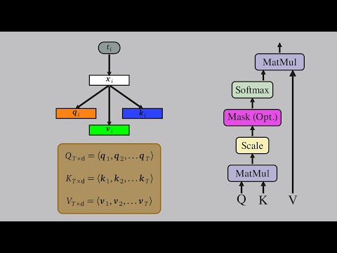
Let's walk step-by-step through self-attention and multi-head attention using a sentence of 6 tokens, an embedding size of 512, and 8 attention heads. This will involve:

• Token embedding
• Sinusoidal positional encoding
• Self-attention computation
• Multi-head attention
• Output vector for predicting the next word

Example Sentence

Let’s take this simple 6-token sentence:

"The cat sat on the mat"

We'll call this S = [t₁, t₂, t₃, t₄, t₅, t₆], where each tᵢ is a token.

Step 1: Token Embedding

Each token is converted to a 512-dimensional vector via a learned embedding table.

• Input tokens (shape): S = (6,)
• Embedding output: E = (6, 512) — 6 tokens, each with 512 features

Example: t₁ = "The" → [0.12, 0.88, ..., 0.55] (512-dim vector) ...same for other tokens.

Step 2: Positional Encoding

Since self-attention has no sense of sequence, we add positional encoding.

• Use sinusoidal encoding of shape (6, 512)

• Each position pos and dimension i is computed as:

  PE(pos, 2i) = sin(pos / 10000^(2i/512))
  PE(pos, 2i+1) = cos(pos / 10000^(2i/512))

Add this to the embedding:

X = E + PE  → shape = (6, 512)

Step 3: Linear Projections (Q, K, V)

For each token, we compute:

• Query (Q): what am I looking for?
• Key (K): what do I contain?
• Value (V): what info do I pass on?

We have weight matrices for each:

Wq, Wk, Wv ∈ ℝ⁵¹²ˣ⁶⁴ (because 512 / 8 = 64 per head)

So for each head:

Q = X @ Wq   → shape (6, 64)
K = X @ Wk   → shape (6, 64)
V = X @ Wv   → shape (6, 64)

Step 4: Scaled Dot-Product Attention (Per Head)

For each token i, compute attention to every token j:

score(i, j) = (Q[i] · K[j]) / √64

This gives a score matrix of shape (6, 6) (Each token attends to every other token including itself.)

Apply softmax across each row → normalize attention weights.

Then multiply weights with V:

Attention[i] = softmax(score[i]) @ V
→ shape = (6, 64)

Step 5: Multi-Head Attention

Do steps 3–4 for all 8 heads in parallel:

• Each head gives a (6, 64) output
• Concatenate all: (6, 8×64) = (6, 512)

Then apply a final linear projection:

Output = (6, 512) @ Wₒ (where Wₒ ∈ ℝ⁵¹²ˣ⁵¹²)

Step 6: Predicting the Next Word

The output (6, 512) is passed through:

• Possibly a feedforward layer (2-layer MLP)
• Then a softmax layer over the vocabulary

We only take the final token's output vector:

x₆ = Output[5] → (512,)

Project it to vocab size (e.g., 50,000):

logits = x₆ @ W_vocab.T → (50,000,)
next_word = softmax(logits)

Summary of Shapes

Would you like me to visualize these with matrices and real numbers or build a small Python simulation of this with dummy data?

CODE

You just ran a simplified single-head self-attention mechanism in Python using a 6-token sequence, each with a 512-dim embedding split into 64-dim heads.

Here's what the code did:

• Generated dummy 512-dim token embeddings
• Added sinusoidal positional encodings
• Computed Q, K, V matrices using learned weights
• Applied scaled dot-product attention
• Visualized attention scores between all token pairs
• Printed the attention output vector of the first token

Next Steps:

Would you like:

1. Full multi-head attention with all 8 heads and output concatenation?
2. Or step-by-step breakdown with real words and embedding simulation (optional for deeper insight)?
3. Or building a prediction layer on top (softmax logits over dummy vocab)?

Let me know how deep you want to go!

MORE

Here’s what you’ve just accomplished through this multi-head attention pipeline:

✅ Complete Workflow Summary

1. Sentence Representation Simulated a 6-token sentence with 512-dim learned embeddings.

2. Positional Encoding Added sinusoidal positional vectors to give the model sequence awareness.

3. Q, K, V Projections (8 heads) Projected each token into 8 different Query, Key, Value spaces using learned weights:

   • Q, K, V shapes: (6, 64) per head

4. Self-Attention (Head-wise)

   • For each head, calculated scaled dot-product attention across all token pairs.
   • Weighted the values V and collected attention outputs.

5. Concatenation & Linear Projection

   • Combined all 8 heads → shape (6, 512)
   • Projected through final output linear layer.

6. Feedforward Neural Network

   • Simulated a 2-layer FFN (ReLU) → (6, 512)

7. Vocabulary Projection & Softmax

   • Used the last token’s output vector to generate probabilities over a 10,000-word dummy vocabulary.

📈 Visualization

You saw a heatmap of attention weights for Head 0, showing how each token attends to others.

🔮 Output

The top 5 "predicted" tokens (just dummy token indices here):

Token indices: [3273, 9999, 3330, 3337, 3336]
Probabilities: [1. 0. 0. 0. 0.]

The top prediction is token 3273, since we only used random weights — the real model would train these over time using backpropagation and loss.

Would you like:

• An interactive version using real words and embeddings (e.g., with Hugging Face)?
• Export to a PDF/PPT explaining this entire pipeline with diagrams?
• Or the same for Transformer encoder block including layer normalization?

Let me know!

INTERACTIVE

Great! Let’s build an interactive self-attention visualizer using real words and embeddings with 🤗 Hugging Face Transformers and torch.

You’ll:

• Use a real model like bert-base-uncased
• Tokenize a sentence (like “The cat sat on the mat”)
• Extract Q, K, V from a specific layer/head
• Visualize attention scores
• Interactively explore the attention of each word

✅ Run the following in Google Colab

🔧 Step 1: Install Required Packages

!pip install transformers torch matplotlib seaborn --quiet

🧠 Step 2: Load the Model and Tokenizer

import torch
from transformers import BertTokenizer, BertModel
import seaborn as sns
import matplotlib.pyplot as plt

# Load BERT base model and tokenizer
model_name = 'bert-base-uncased'
tokenizer = BertTokenizer.from_pretrained(model_name)
model = BertModel.from_pretrained(model_name, output_attentions=True)
model.eval()

📝 Step 3: Encode Your Sentence

sentence = "The cat sat on the mat"
inputs = tokenizer(sentence, return_tensors='pt')
with torch.no_grad():
    outputs = model(**inputs)

# Get attention from all layers and heads
attentions = outputs.attentions  # Tuple of 12 layers, each (1, 12, seq_len, seq_len)
tokens = tokenizer.convert_ids_to_tokens(inputs['input_ids'][0])

🔍 Step 4: Visualize Attention from a Layer and Head

# Choose layer and head
layer_num = 0  # 0 to 11
head_num = 0   # 0 to 11

attn = attentions[layer_num][0, head_num]  # (seq_len, seq_len)

# Plot
plt.figure(figsize=(8, 6))
sns.heatmap(attn, xticklabels=tokens, yticklabels=tokens, cmap="Blues", annot=True, fmt=".2f")
plt.title(f"Layer {layer_num + 1} Head {head_num + 1} Attention")
plt.xlabel("Key")
plt.ylabel("Query")
plt.show()

🧪 Try Changing:

• layer_num and head_num to explore other heads/layers
• Input sentence (even longer ones)
• Use multiple attention heads at once

Would you like this wrapped into a Streamlit app or Gradio UI to allow sliders/dropdowns for real-time interaction?

Or exported as a Colab notebook link or PPT/PDF visual explanation of what you just explored?

ATTENTION IS ALL YOU NEED

Here’s an approachable walkthrough of “Attention Is All You Need” (Vaswani et al., 2017), the paper that introduced the Transformer—and how its ideas evolved into GPT-2 and other modern models.

1. Motivation: Why Move Beyond RNNs/CNNs?

• Sequential bottleneck: RNNs process tokens one at a time, making it hard to parallelize and to capture long-range dependencies.
• Fixed-size kernel: CNNs need many layers or large kernels to see far apart tokens.
• Solution: A pure “attention” mechanism that directly links every input and output position, letting the model learn which tokens to focus on—fully parallelizable and flexible in range.

2. Core Building Block: Scaled Dot-Product Attention

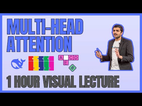
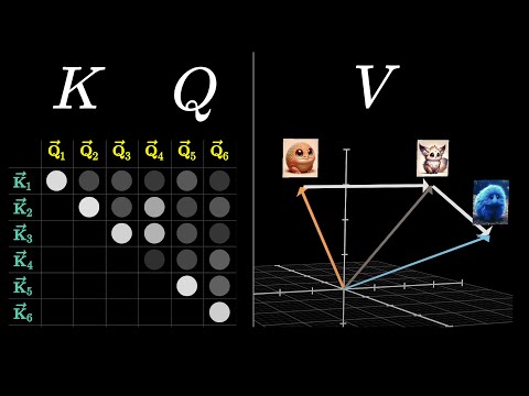
Given queries Q, keys K, and values V (all matrices):

Attention(Q,K,V) = softmax( QKT / √dₖ ) · V

• QKT computes similarity between each query and all keys.
• Dividing by √dₖ (the key dimensionality) stabilizes gradients.
• The softmax turns similarities into weights (i.e., attention scores).
• Multiplying by V aggregates information from all positions.

3. Multi-Head Attention

Instead of one attention, use h separate “heads”:

1. Linearly project Q, K, V into h subspaces (lower dimensional).
2. Apply scaled dot-product attention in each head in parallel.
3. Concatenate the heads’ outputs and project back to the model dimension.

Why multi-head?

• Different heads can learn to focus on different types of relationships (e.g., syntax vs. semantics).
• Increases modeling power without blowing up computation.

4. Adding Order: Positional Encoding

Since attention alone is order-agnostic, the paper adds sinusoidal positional encodings to the input embeddings:

PE(pos,2i)   = sin(pos / 10000^(2i/d_model))
PE(pos,2i+1) = cos(pos / 10000^(2i/d_model))

• Injects unique, smooth position signals.
• Enables the model to learn relative and absolute positions.

5. Position-wise Feed-Forward Networks

Each encoder/decoder layer includes a small fully-connected network applied to each position separately:

FFN(x) = max(0, xW₁ + b₁)W₂ + b₂

• Two linear layers with a ReLU in between.
• Same parameters shared across all positions.

6. Encoder & Decoder Stacks

• Encoder: A stack of N identical layers, each with

  1. Multi-head self-attention over the input sequence.
  2. Feed-forward network.

• Decoder: Also N layers, but each layer has

  1. Masked multi-head self-attention over target (prevents peeking at future tokens).
  2. Multi-head attention over encoder outputs (to attend to source).
  3. Feed-forward network.

Each sub-layer has a residual connection + layer normalization:

LayerNorm(x + SubLayer(x))

This stabilizes training and helps gradient flow.

7. Full Forward Pass

1. Input tokens → embeddings + positional encodings.
2. Pass through the N encoder layers → final encoder representations.
3. Decoder: start with “” → embeddings + positional encodings → through N decoder layers, attending to encoder outputs.
4. Final decoder output → linear + softmax → probability distribution over vocabulary for next token.

Because every layer is fully parallelizable (no recurrence), training is much faster on GPUs/TPUs.

8. Relation to GPT-2 (and “So On”)

GPT-2 (Radford et al., 2019) builds directly on the Transformer decoder:

Why decoder-only?

• For language modeling, you only need to predict each token from previous tokens.
• Dropping the encoder simplifies the model and speeds inference.

Evolution Beyond GPT-2

• GPT-3/3.5/4: scale up layer count, width, data, and training compute.
• BERT: encoder-only Transformer, trained with masked LM objective for bidirectional context.
• T5: full encoder–decoder trained on a “text-to-text” framework, extending Transformers to any NLP task.
• Transformer-XL, Longformer, etc.: introduce recurrence or sparse/linear attention to handle longer contexts.

Why This Matters

• The pure-attention design freed NLP from sequential processing constraints.
• It set the stage for ever-larger models (GPT family, BERT, T5) simply by scaling layers, width, and data.
• Variants tailor the basic blocks—self-attention, feed-forward, residual connections—to different objectives (generation, classification, translation).

In sum, “Attention Is All You Need” replaced RNNs/CNNs with a fully parallel, attention-centric architecture. GPT-2 is a direct descendant that prunes away the encoder, uses causal masking for text generation, and scales up massively in size—and the same core ideas power most state-of-the-art NLP models today.

When you read “project into lower-dimensional subspaces,” it doesn’t contradict the fact that in code you often see a single 768→2304 linear layer for QKV. Here’s what’s really happening:

1. Model vs. head dimension

   • d_model: the hidden size of your transformer (e.g. 768 in GPT-2-small).
   • h: number of heads (12 for GPT-2-small).
   • d_k = d_model / h: the size of each head’s subspace (768 / 12 = 64).

2. Combined QKV projection (768 → 2304)

   • For efficiency, frameworks pack the three projections into one matrix:

     $$ W{\text{inproj}} \in \mathbb{R}^{d{!model}\times 3d{!model}} \quad:\quad X\,W{\text{inproj}} ~\in~ \mathbb{R}^{\text{seq}\times 3d_{!model}} $$

   • Numerically, 768×2304 = three copies of 768, one each for Q, K and V.

3. Splitting into Q, K, V

   • You slice that 2304-dim vector into three 768-dim chunks:

     $$ [Q{\text{flat}},\,K{\text{flat}},\,V_{\text{flat}}] ~\in~ \mathbb{R}^{\text{seq}\times 768}\;\times3 $$

4. Reshaping into h heads (lower-dimensional!)

   • Each 768-dim vector is then reshaped to (h, d_k):

     $$ 768 \;\longrightarrow\; (12 \times 64) \quad\text{so each head has dimension } d_k=64. $$

   • Now your queries, keys, and values live in twelve 64-dim subspaces, each much smaller than 768.

Why split into lower-dimensional heads?

• Constant compute: If you did 12 heads each of size 768, you’d multiply your FLOPs by 12. By making each head size 64, the total cost stays

  $$ h \times (\text{seq}^2 \times dk) = \text{seq}^2 \times (h\cdot dk) = \text{seq}^2 \times d_{!model}. $$

• Specialization: Different heads can focus on different kinds of relationships (syntax vs. semantics, local vs. global patterns), improving representational power without extra cost.

• Stable optimization: Lower-dim dot products (64‐dimensional) have smaller variance than huge 768-dim ones, which helps training.

In short:

• The “768 → 2304” you saw is just a combined QKV projection for efficiency.
• The true “lower‐dimensional” step is when each of those 768-dim Q, K, V vectors is split into 12 heads of size 64.
• That’s why the paper says “project into h subspaces (lower dimensional)”—each head really is smaller than the original hidden size.

Under the hood, the step that takes your 768-dimensional token embedding x and turns it into the concatenated Q, K, V vector is simply a single linear transformation:

1. Combined projection weight You have a learned weight matrix

   $$ W{\text{inproj}}\;\in\;\mathbb R^{\,d{!model}\,\times\,3\,d_{!model}} \;=\;\mathbb R^{768\times(3\times768)} \;=\;\mathbb R^{768\times2304} $$

   and a bias vector

   $$ b_{\text{inproj}}\;\in\;\mathbb R^{2304}. $$

2. Linear map When you apply it to your embedding

   $$ x\in\mathbb R^{768}, $$

   you compute

   $$ \bigl[xW{\text{inproj}} + b{\text{inproj}}\bigr]\;\in\;\mathbb R^{2304}. $$

   That 2304-dim vector is literally $[Q{\mathrm{flat}}\;|\;K{\mathrm{flat}}\;|\;V_{\mathrm{flat}}]$, three 768-dim slices stuck end to end.

3. Why 2304 (not 2308)? The standard Transformer always uses exactly $3\times d_{!model}$. If you saw “2308” it’s either a typo or comes from a custom variant that padded or added extra parameters—but the vanilla Vaswani et al. model is $3\times768=2304$.

4. Splitting into Q, K, V In code you’ll see something like (PyTorch-style):

   # in_proj_out: [batch, seq_len, 2304]
   in_proj_out = linear(x, W_inproj, b_inproj)
   # now split into three 768-dim tensors
   Q_flat, K_flat, V_flat = in_proj_out.chunk(3, dim=-1)

5. Reshaping for multi-head Each of those 768-dim vectors is then reshaped into your h heads of size dₖ = 768/ h (e.g. 12 heads of 64 dims):

   # from [batch, seq_len, 768] → [batch, h, seq_len, d_k]
   Q = Q_flat.view(batch, seq_len, h, d_k).transpose(1,2)
   # same for K and V

In summary:

• One Linear layer of shape (768 → 2304) creates the concatenated QKV.
• You then slice that 2304 vector into three 768-dim heads.
• Finally, you reshape into h subspaces of size dₖ = 768/h, giving you your “lower-dimensional” per-head Q, K, and V.